Matrix Operations in Machine Learning

One of the interesting things to play around machine learning is to optimize the computational cost in training the learning model through matrix operations.

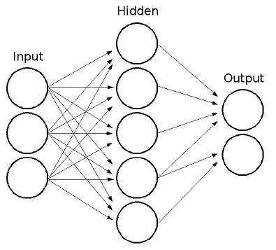
Taking a 3 layers neuron network as an example, it has one input layer, one hidden layer and one output layer, it is a typical model being used for recognizing handwritten numbers as shown below.

Without using matrix operation, one can loop through K training samples to compute the output in layer 2 and 3, and finally get the summation of the total cost J. This code is more concise and easy to understand.

J = 0; % J is the cost of the network

for i = 1:K % K is the number of training samples

  % layer 1

  a1 = X(i,:); % X is the input features 

  % layer 2

  z2 = Theta1 * a1'; % Theta1

  a2 = sigmoid(z2); % sigmoid is logistic function

  % layer 3

  z3 = Theta2 * [1; a2]; % Theta2 is 

  a3 = sigmoid(z3);

  % yy is the output

  J += -yy(i,:)*log(a3)-(1-yy(i,:))*log(1-a3);

end

J = J / K;

If we implemented it with matrix operation without looping through K training sample, we can leverage the code optimization through matrix operation and eliminate the for loop. I got 2.x times faster on my machine. (without seriously benchmarking the performance)

all_z2 = Theta1 * X';

all_a2 = sigmoid(all_z2);

all_a2 = [ones(1, K); all_a2];

all_z3 = Theta2 * all_a2;

all_a3 = sigmoid(all_z3);

J = 0;

for i = 1:K

  J += -yy(i,:)*log(all_a3(:,i))-(1-yy(i,:))*log(1-all_a3(:,i));

end

J = J / K;

However, if we blindly to use matrix operations as shown below, it introduces 2*K*K - K redundant operations, making it even runs slower than the first implementation above.

all_a31 = -yy * log(all_a3) .* eye(K);
all_a32 = (1 - yy) * log(1 - all_a3) .* eye(K);
all = all_a31 - all_a32;
J = sum(sum(all));